Decoding Metastatic Potential in Colorectal Cancer Using Tissue Cytometry

As a part of ASI 2025 Lunch and Learn Session, Dr Melanie McCoy and Ms Tracey Lee-Pullen presented their research on metastatic colorectal cancer. Using quantitative tissue cytometry, the team aims to investigate if the tumor microenvironment predicts metastasis development. For quantification of pre-determined T lymphocyte subsets, the researchers employed StrataQuest image analysis solution from TissueGnostics.

Webinar Transcript

Dr Melanie McCoy

Okay, I’m just going to briefly introduce who we are and what we do, and then I’m going to hand over to Tracy to do all the work.
[laughter]

Tracy and I are part of the colorectal cancer research group at St John of God Hospital here in Perth. This is who we are, and these are our main areas of interest. Most of our work focuses on identifying immune-related biomarkers of prognosis or treatment response in colorectal cancer. Quantitating cells in tissue is central to what we do.

Back in 2017, we were lucky enough to receive funding for image analysis software. At the time, we looked at the systems that were available and settled on StrataQuest. Initially, Tracy and I were drawn to StrataQuest because we both come from a flow cytometry background. The flow-style gating and back-gating that Robert just presented really appealed to us. We also loved how customizable the software appeared to be and how strong the customer support seemed.

We’ve used StrataQuest for all of our image analysis since then, and Tracy is going to talk about one of our most recent projects that used StrataQuest, as well as share some of the tips and tricks we’ve learned along the way.

MS Tracey Lee-Pullen

Hopefully I’ll share some useful tips.

As Mel just alluded to, my previous life was as a flow cytometrist. I’m not sure I can still call myself that, given that I haven’t touched a flow cytometer in about four years, because now I work with images. I should also say that I’m not an immunologist either, so I suppose I can just say I’m a cytometry nerd now.

I worked for six and a half years in a core facility at the Centre for Microscopy, Characterisation and Analysis at UWA, where I did a lot of flow cytometry and microscopy. When I moved into the research group at St John’s, it seemed to fit quite well to move into the imaging cytometry space as well.

I should also note that when I first saw the scattergrams Robert presented, I was a bit skeptical as a flow cytometrist. But they’re incredibly powerful, very useful, and they work very well.

To give you a bit of context, the project I’m going to talk about today is actually the PhD project of this very smiley, happy guy here called Ryan, who is not quite so smiley and happy at the moment because he’s currently in a surgical training program. Otherwise, he would be here today.

His project is focused on the role of the tumor microenvironment in metastasis development. The question is: can we see a difference in tumors at the time of resection that might indicate whether they have a higher risk of recurrence?

To do this, and you’ll hear lots of talks this week and last week at the cytometry meeting about much higher-parameter panels, this is actually a relatively simple project. We don’t have access to a spectral scanning system here in Perth, so we designed a panel to be run on a standard immunofluorescent staining system. We did get it working on the Bond automated stainer, much to Ryan’s delight, because it turned the process into an overnight run rather than a two-day one.

StrataQuest is where I came in, helping to turn all of this into meaningful data.

Background: Colorectal Cancer and Metastasis

Colorectal cancer, which Mel mentioned, is one of the most common cancers in Australia and also has one of the highest mortality rates. We often don’t detect colorectal cancer until it is too late.

Colorectal cancer develops in the colon and rectum and progresses through different stages of invasion. It starts in the mucosa and then moves through stages such as T1 and T2 as it invades deeper into the bowel wall. Eventually, once it leaves the bowel wall, it may spread to the regional lymph nodes and then to distant sites, most commonly the liver and lungs.

The stage depends on the level of invasion and where the cancer has spread. For the purposes of Ryan’s project:

• Stages 1 to 3 are classified as the non-metastatic group
• Stage 4 is the distant metastasis group

For bowel cancer treatment, management often depends on the location and severity of the disease. Many colon cancer patients go straight to surgery, and then, depending on the pathology findings and whether the disease is metastatic, they may receive adjuvant therapy afterward.

Then comes the waiting game: if the tumor has been successfully removed, will the patient develop a recurrence? Unfortunately, one in three patients will develop recurrence, either locally or as distant metastasis.

The term used here is metachronous metastasis — meaning metastasis that develops later, often within five years of surgery. For some patients, we already know they are at higher risk based on their clinical information and pathology. In fact, for about 60% of patients who develop recurrence, we already have some indication that recurrence is likely. But for roughly 40%, we do not know in advance that they are high risk. These are the patients we may want to monitor more closely or potentially offer adjuvant therapy to if they were not already indicated for it.

Project Aim

Ryan’s project focuses on the tumor microenvironment, particularly the local immune profile within these tumors. The idea is that there may be a different immune landscape in tumors that later develop metastasis.

The project uses a couple of panels focused on lymphocytes. The one I’m discussing today includes a tissue-resident marker. The aim is to evaluate the local immune response in the resected tumor and determine whether there is an association between immune phenotype and later metastasis.

Study Design

Ryan’s study is a nested case-control study using patients who underwent surgery between 2010 and 2020.

The main group of interest is the metachronous metastasis group. These are patients who, at the time of surgery, had local or locally advanced tumors with no detectable metastases in the liver or lungs, but who then developed metastatic recurrence within five years.

The control group includes patients who also had no metastases at the time of surgery and did not develop recurrence. These control patients were matched to the recurrence group by characteristics such as:

• age
• sex
• stage
• treatment

The third group is the synchronous metastasis group — patients who already had metastasis at the time of surgery. These serve as a kind of positive control because we already know they have progressed to stage 4 disease.

Sample Workflow

This meeting will showcase a lot of exciting data, but today I’m not showing data. Instead, I’m focusing on how we do what we do.

The samples we use are human FFPE tissues taken from pathology archives. We create tissue microarrays (TMAs), then perform staining, imaging, and quantitation.

We start with tissue blocks from tumor resections. Often there are multiple blocks per case. Our pathologist reviews them and carefully marks different areas of interest:

• the leading edge of the tumor
• the central tumor
• the normal mucosa

We then align those marked areas, punch cores out, and place them into a TMA block. Sometimes this works more successfully than others.

As a result, we produce TMAs that ideally look like neat grids, although anyone who has worked with TMAs knows that they do not always behave that way. Entire columns can drift, and sometimes the tumor is not hit exactly where intended. Some cases may also be responders to treatment, so the tissue composition can vary.

For each patient, we take:

• two normal cores
• two invasive margin cores
• two central tumor cores

We do this because:

1. sometimes we miss the tumor, and
2. the staining process is quite harsh on the tissue, so cores can be lost.

We also take serial sections for the project, including an H&E stain for all fluorescent slides so we can refer back to morphology during annotation.

Staining Workflow

The staining was performed on the Bond RX system, which improved reproducibility and reduced variation. However, we found that TMA size mattered. If the TMAs were too large, we could get edge effects due to solution flow through the system. So we kept the TMAs smaller and asymmetric, which also helped with orientation.

The staining method we used is TSA (tyramide signal amplification). In this system:

1. the primary antibody binds
2. a secondary HRP reagent is added
3. a fluorophore-linked tyramide is deposited

This is useful because it gives signal amplification, which increases sensitivity. It also allows us to perform another retrieval step afterward, strip off the antibodies, and then apply another primary antibody raised in the same species.

That was one of the main reasons we initially looked at TSA: it let us use multiple antibodies from the same host species. An added benefit was signal amplification, which helped with our colorectal tissue, where high collagen content leads to high autofluorescence.

We initially hoped to get six colors from the system, but to obtain reliable data, we settled on five. That may sound low compared with some current approaches, but we preferred robust, accurate data over pushing the panel too far.

Optimization

I won’t dwell too much on the optimization, but it was a major part of the project. Ryan actually wrote up the methods because he probably spent 80% of his time optimizing and only 20% actually doing the staining.

The optimization process included:

• testing antigen retrieval methods
• titrating the primary antibodies
• checking the secondary detection reagents
• assessing whether antibodies could be stripped effectively
• assigning the correct fluorophores
• determining the correct staining order

The staining order was especially important.

One challenge is that we are working with human pathology samples, so we have no control over how long the tissue sat in formalin before processing. Unlike mouse experiments, where fixation can be tightly controlled, surgical specimens may sit for varying lengths of time before entering the pathology workflow. This affected fluorescence intensity for some markers.

Another challenge was tissue integrity. During repeated stripping rounds, the tissue is essentially heated to very high temperatures multiple times. Slide choice turned out to be very important. We used a very adhesive slide type that helped keep the tissue attached.

We also had some issues with antibody stripping. Most markers stripped off well, but CD103 did not strip effectively. Rather than endlessly trying new stripping methods, we adjusted the staining order so that CD103 was placed at the end, where incomplete stripping would not interfere.

Similarly, the Polaris 780 fluorophore also had to go at the end, so these two considerations had to be worked into the same staining sequence.

Imaging

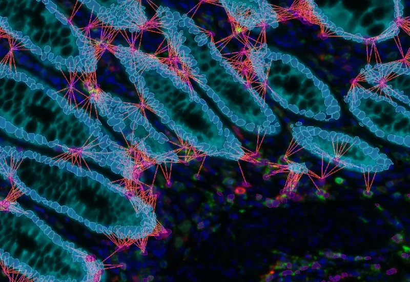
The imaging was done on a standard fluorescent scanner with band-pass filters and an LED light engine. We designed the panel to work within those constraints. With a spectral system we might have been able to push to seven colors, but we were very happy with the five-color panel because it gave us good separation without crosstalk.

The result is a very beautiful image — even if it is, unfortunately, cancer.

We can clearly see:

• tumor-infiltrating lymphocytes
• stromal T cells

And that brings us to the step where we need to convert those images into numbers.

Image Analysis in StrataQuest

For this project, we were interested in:

• the density of different cell populations
• where those cells are located within the tissue

The original analysis was performed in StrataQuest version 1.29, which is an older version than the one shown earlier today. I mention that because I’ll also briefly show how the new version improves nuclear segmentation.

What I’m doing today may look complex because I now build my own analysis apps. But when we first got the software, we simply gave the team our stains, our markers, and our questions, and they designed the analysis profile for us. That allowed us to start using the software immediately through an easy user interface. Since then, I’ve become the sort of person who pulls things apart, rebuilds them, and teaches herself to make custom apps and profiles.

One nice feature is that I can also simplify those profiles for students and collaborators, so they can run analyses using just a few buttons while still relying on a more sophisticated underlying setup.

Analysis Workflow

My process usually is:

1. open the file
2. segment the TMA cores
3. classify tissue masks
4. segment the cells
5. identify cell phenotypes

TMA Segmentation

TMA segmentation is quite straightforward. The software can auto-detect the tissue, but we still tend to create a grid manually because we have an Excel map of the TMA layout. If every possible core position is included, the exported data overlays neatly with that map.

Our TMA is asymmetric, which helps us orient it correctly on the slide.

These regions allow us to apply analysis across the whole slide while still exporting data separately for each core.

Tissue Masks

We typically create three masks:

• a tissue mask
• an epithelial mask
• a stromal mask

These allow us to:

• limit the analysis to tissue only
• calculate areas for density measurements
• classify cells as epithelial or stromal

For the tissue mask, the software can auto-detect tissue, but we still inspect it manually. We want to exclude things like:

• tissue folds
• debris
• luminal contents

These can otherwise distort the results.

For the epithelial mask, we use a pan-cytokeratin marker to identify epithelium. We then threshold and clean up that signal to create the epithelial mask. Everything outside that becomes stroma.

This allows us to quantify cells in:

• the whole tissue
• the epithelium
• the stroma

We can also create distance bands from the epithelium and examine how cell populations vary with distance.

Nuclear Segmentation

This part is critically important. Anyone who works in this area knows that one of the main questions is: what actually counts as a cell?

There are always caveats. We’re looking at 2D sections and TMAs, so we are never going to achieve perfect segmentation. As someone coming from flow cytometry, that required a real lesson in accepting imperfection. But there are a lot of things we can do to reduce error.

Our samples are challenging because colorectal tumors contain a wide range of nuclear shapes and sizes:

• tumor nuclei can be elongated
• lymphocytes are often small and round
• stromal lymphocytes can be stretched
• densely packed lymphocyte areas are difficult to separate

We optimized our settings to better identify lymphocytes, since they were our main interest, rather than focusing on perfect segmentation of tumor nuclei.

With the newer software version and deep neural network (DNN)-based nuclear segmentation, we now get:

• tighter nuclear masks
• rounder segmentation
• better separation of adjacent cells
• less over-segmentation

There is still some imperfection, but it is a major improvement.

Cell Masks and Phenotyping

Once a nucleus is identified, we create a cell mask by expanding the nuclear mask outward and inward slightly. This gives us a region where we can examine cell surface markers.

To decide how far to expand that mask, I compare it directly against markers such as CD3 to make sure the membrane-associated signal is captured appropriately.

For each cell mask, the software can extract a wide range of measurements, including:

• mean fluorescence intensity
• upper-percentile intensity
• size
• area of signal

Originally, we used the mean intensity for gating. For example, we could plot:

• CD3 mean intensity
• versus CD8 mean intensity

Then we could set gates and back-gate to see where those cells are in the tissue.

One very nice feature is the ability to validate the gating visually. The software can bring up individual cell images so you can scroll through them and judge whether your threshold is sensible.

For double-positive populations, such as CD3+CD8+ cells, we can gate on the upper-right quadrant and identify those cells.

However, because I’m naturally skeptical, especially when dealing with rare subsets, I wanted to be sure that a double-positive or triple-positive signal really represented a single positive cell — not just adjacent cells whose signal had been partially captured in the same mask.

So I developed an approach using threshold masks. For each marker, I create a binary mask where pixels above a certain intensity threshold are marked. I then overlay these masks. Wherever the overlap is present, I know that both markers are truly co-localized. I can then measure how much of that overlap falls inside the cell membrane mask. This gives me more confidence, especially for double- and triple-positive populations.

The difference may seem subtle visually, but it gives me much more confidence that I am identifying true co-expression rather than accidental proximity.

Outputs

At the end of the project, we obtain:

• total counts of CD3+ cells
• CD3+CD8+ cells
• CD3+CD103+ cells
• triple-positive populations

We can measure these populations within:

• the whole tissue mask
• the epithelial mask
• the stromal mask

We also calculate the areas of those compartments, which allows us to derive cell densities.

Because of the hierarchical gating, we can also calculate proportions, not just counts. For example, we can determine what proportion of CD8 cells express CD103.

Closing Remarks

The overall aim was to determine whether there is a distinct immune subset in the metachronous metastasis group.

We used this five-color panel, together with additional panels, and analyzed the samples in StrataQuest. We do have some preliminary data, which will be presented on a poster on Thursday. So if you’d like to see what we actually found, please come along and have a look.